23 Feb 2017
Editor’s note: This is the fourth chapter of a book I’m working on called Demystifying Artificial Intelligence. I’ve also added a co-author, Divya Narayanan, a masters student here at Johns Hopkins! The goal of the book is to demystify what modern AI is and does for a general audience. So something to smooth the transition between AI fiction and highly mathematical descriptions of deep learning. We are developing the book over time - so if you buy the book on Leanpub know that there are only four chapters in there so far, but I’ll be adding more over the next few weeks and you get free updates. The cover of the book was inspired by this amazing tweet by Twitter user @notajf. Feedback is welcome and encouraged!
“A learning machine is any device whose actions are influenced by past experience.” - Nils John Nilsson
Machine learning describes exactly what you would think: a machine that learns. As we described in the previous chapter a machine “learns” just like humans from previous examples. With certain experiences that give them an understanding about a particular concept, machines can be trained to have similar experiences as well, or at least mimic them. With very routine tasks, our brains become attuned to characteristics that define different objects or activities.
Before we can dive into the algorithms - like neural networks - that are most commonly used for artificial intelligence, lets consider a real example to understand how machine learning works in practice.
The Big One
Earthquakes occur when the surface of the Earth experiences a shake due to displacement of the ground, and can readily occur along fault lines where there have already been massive displacements of rock or ground(Wikipedia 2017a). For people living in places like California where earthquakes occur relatively frequently, preparedness and safety are major concerns. One famous fault in southern California, called the San Andreas Fault, is expected to produce the next big earthquake in the foreseeable future, often referred to as the “Big One”. Naturally, some residents are concerned and may like to know more so they are better prepared.
The following data are pulled from fivethirtyeight, a political and sports blogging site, and describe how worried people are about the “Big One” (Hickey 2015). Here’s an example of the first few observations in this dataset:
| |
worry_general |
worry_bigone |
will_occur |
| 1004 |
Somewhat worried |
Somewhat worried |
TRUE |
| 1005 |
Not at all worried |
Not at all worried |
FALSE |
| 1006 |
Not so worried |
Not so worried |
FALSE |
| 1007 |
Not at all worried |
Not at all worried |
FALSE |
| 1008 |
Not at all worried |
Not at all worried |
FALSE |
| 1009 |
Not at all worried |
Not at all worried |
FALSE |
| 1010 |
Not so worried |
Somewhat worried |
FALSE |
| 1011 |
Not so worried |
Extremely worried |
FALSE |
| 1012 |
Not at all worried |
Not so worried |
FALSE |
| 1013 |
Somewhat worried |
Not so worried |
FALSE |
Just by looking at this subset of the data, we can already get a feel for how many different ways it could be structured. Here, we see that there are 10 observations which represent 10 individuals. For each individual, we have information on 11 different aspects of earthquake preparedness and experience (only 3 of which are shown here). Data can be stored as text, logical responses (true/false), or numbers. Sometimes, and quite often at that, it may be missing; for example, observation 1013.
So what can we do with this data? For example, we could predict - or classify - whether or not someone was likely to have taken any precautions for an upcoming earthquake, like bolting their shelves to the wall or come up with an evacuation plan. Using this idea, we have now found a question that we’re interested in analyzing: are you prepared for an earthquake or not? And now, based on this question and the data that we have, we can see that you can either be prepared (seen above as “true”) or not (seen above as “false”).
Our question: How well can we predict whether or not someone is prepared for an earthquake?
An Algorithm – what’s that?
With our question in tow, we want to design a way for our machine to determine if someone is prepared for an earthquake or not. To do this, the machine goes through a flowchart-like set of instructions. At each fork in the flowchart, there are different answers which take the machine on a different path to get to the final answer. If you go through the correct series of questions and answers, it can correctly identify a person as being prepared. Here’s a small portion of the final flowchart for the San Andreas data which we will proceed to dissect (note: the ellipses on the right-hand side of the flowchart indicate where the remainder of the algorithm lies. This will be expanded later in the chapter):
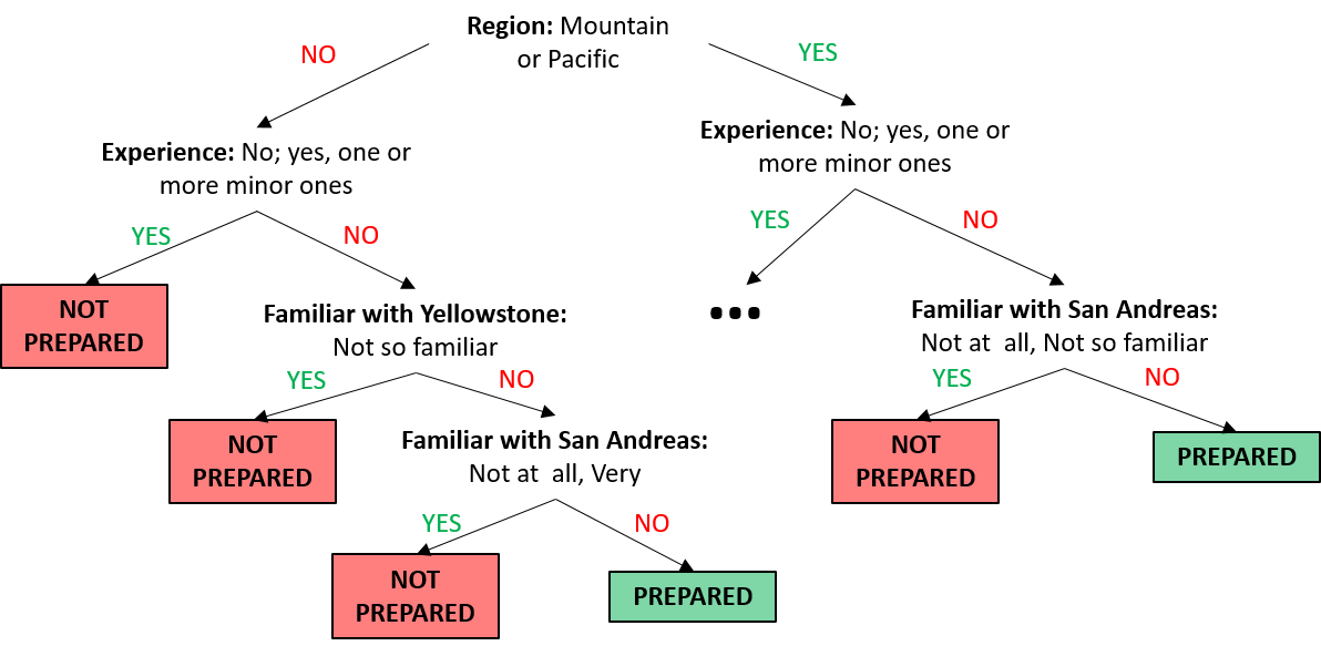
The steps that we take through the flowchart, or tree make up the classification algorithm. An algorithm is essentially a set of step-by-step instructions that we follow to organize, or in other words, to make a prediction about our data. In this case, our goal is to classify an individual as prepared or not by working our way through the different branches of the tree. So how did we establish this particular set of questions to be in our framework of identifying a prepared individual?
CART, or a classification and regression tree, is one way to assess which of these characteristics is the most important in terms of splitting up the data into prepared and unprepared individuals (Wikipedia 2017b, Breiman et al. (1984)). There are multiple ways of implementing this method, often times with the earlier branches making larger splits in the data, and later branches making smaller splits.
Within an algorithm, there exists another level of organization composed of features and parameters.
In order to tell if someone is prepared for an earthquake or not, there have to be certain characteristics, known as features, that separate those who are prepared from those who are not. Features are basically the things you measured in your dataset that are chosen to give you insight into an individual and how to best classify them into groups. Looking at our sample data, we can see that some of the possible features are: whether or not an individual is worried about earthquakes in general, prior experiences with earthquakes, or their gender. As we will soon see, certain features will carry more weight in separating an individual into the two groups (prepared vs. unprepared).
If we were looking at how important previously experiencing an earthquake was in classifying someone as prepared, we’d say it plays a pretty big role, since it’s one of the first features that we encounter in our flowchart. The feature that seems to make a bigger split to our data is region, as it appears as the first feature in our algorithm shown above. We would expect that people in the Mountain and Pacific regions have more experience and knowledge about earthquakes, as that part of the country is more prone to experiencing an earthquake. However, someone’s age may not be as important in classifying a prepared individual. Since it doesn’t even show up in the top of our flowchart, it means it wasn’t as crucial to know this information to decide if a person is prepared or not and it didn’t separate the data much.
The second form of organization within an algorithm are the questions and cutoffs for moving one direction or another at each node. These are known as parameters of our algorithm. These parameters give us insight as to how the features we have established define the observation we are trying to identify. Let us consider an example using the feature of region. As we mentioned earlier, we would expect that those in the Mountain and Pacific regions would have more experience with earthquakes, which may reflect in their level of preparedness. Looking back at our abbreviated classification tree, the first node in our tree has a parameter of “Mountain or Pacific” for the feature region, which can be split into “yes” (those living in one of these regions) or “no” (living elsewhere in the US).
If we were looking at a continuous variable, say number of years living in a region, we may set a threshold instead, say greater than 5 years, as opposed to a yes/no distinction. In supervised learning, where we are teaching the machine to identify a prepared individual, we provide the machine multiple observations of prepared individuals and include different parameter values of features to show how a person could be prepared. To illustrate this point, let us consider the 10 sample observations below, and specifically examine the outcome, preparedness, with respect to the features: will_occur, female, and household income.
| |
prepared |
will_occur |
female |
hhold_income |
| 1004 |
TRUE |
TRUE |
FALSE |
$50,000 to $74,999 |
| 1005 |
FALSE |
FALSE |
TRUE |
$10,000 to $24,999 |
| 1006 |
TRUE |
FALSE |
TRUE |
$200,000 and up |
| 1007 |
FALSE |
FALSE |
FALSE |
$75,000 to $99,999 |
| 1008 |
FALSE |
FALSE |
TRUE |
Prefer not to answer |
| 1009 |
FALSE |
FALSE |
FALSE |
Prefer not to answer |
| 1010 |
TRUE |
FALSE |
TRUE |
$50,000 to $74,999 |
| 1011 |
FALSE |
FALSE |
TRUE |
Prefer not to answer |
| 1012 |
FALSE |
FALSE |
TRUE |
$50,000 to $74,999 |
| 1013 |
FALSE |
FALSE |
NA |
NA |
Of these ten observations, 7 are not prepared for the next earthquake and 3 are. But to make this information more useful, we can look at some of the features to see if there are any similarities that the machine can use as a classifier. For example, of the 3 individuals that are prepared, two are female and only one is male. But notice we get the same distribution of males and females by looking at those who are not prepared: you have 4 females and 2 males, the same 2:1 ratio. From such a small sample, the algorithm may not be able to tell how important gender is in classifying preparedness. But, by looking through the remaining features and a larger sample, it can start to classify individuals. This is what we mean when we say a machine learning algorithm learns.
Now, let us take a closer look at observations 1005, 1011, and 1012, and more specifically the household income feature:
| |
prepared |
will_occur |
female |
hhold_income |
| 1005 |
FALSE |
FALSE |
TRUE |
$10,000 to $24,999 |
| 1011 |
FALSE |
FALSE |
TRUE |
Prefer not to answer |
| 1012 |
FALSE |
FALSE |
TRUE |
$50,000 to $74,999 |
All three of these observations are females and believe that the “Big One” won’t occur in their lifetime. But despite the fact that they are all unprepared, they each report a different household income. Based on just these three observations, we may conclude that household income is not as important in determining preparedness. By showing a machine different examples of which features a prepared individual has (or unprepared, as in this case), it can start to recognize patterns and identify the features, or combination of features, and parameters that are most indicative of preparedness.
In summary, every flowchart will have the following components:
-
The algorithm - The general workflow or logic that dictates the path the machine travels, based on chosen features and parameter values. In turn, the machine classifies or predicts which group an observation belongs to
- Features - The variables or types of information we have about each observation
- Parameters - The possible values a particular feature can have
Even with the experience of seeing numerous observations with various feature values, there is no way to show our machine information on every single person that exists in the world. What will it do when it sees a brand new observation that is not identified as prepared or unprepared? Is there a way to improve how well our algorithm performs?
Training and Testing Data
You may have heard of the terms sample and population. In case these terms are unfamiliar, think of the population as the entire group of people we want to get information from, study, and describe. This would be like getting a piece of information, say income, from every single person in the world. Wouldn’t that be a fun exercise!
If we had the resources to do this, we could then take all those incomes and find out the average income of an individual in the world. But since this is not possible, it might be easier to get that information from a smaller number of people, or sample, and use the average income of that smaller pool of people to represent the average income of the world’s population. We could only say that the average income of the sample is representative of the population if the sample of people that we picked have the same characteristics of the population.
For example, if we assumed that our population of interest was a company with 1,000 employees, where 200 of those employees make $60,000 each and 800 of them make $30,000 each. Since we have this information on everyone, we could easily calculate the average income of an employee in the company, which would be $36,000. Now, say we randomly picked a group of 100 individuals from the company as our sample. If all of those 100 individuals came from the group of employees that made $60,000, we might think that the average income for an employee was actually much higher than the true average of the population (the whole company). The opposite would be true if all 100 of those employees came from the group making less money - we would mistakenly think the average income of employees is lower. In order to accurately reflect the distribution of income of the company employees through our sample, or rather to have a representative sample, we would try to pick 20 individuals from the higher income group and 80 individuals from the lower income group to get an accurate representation of this company population.
Now heading back to our earthquake example, our big picture goal is to be able to feed our algorithm a brand new observation of someone who answered information about themselves and earthquake preparedness, and have the machine be able to correctly identify whether or not they are prepared for a future earthquake.
One definition of a population could consist of all individuals in the world. However, since we can’t get access to data on all these individuals, we decide to sample 1013 respondents and ask them earthquake related questions. Remember that in order for our machine to be able to accurately identify an individual as prepared or unprepared, it needs to have had some experience seeing some observations where features identify the individual as prepared, as well as some observations that aren’t. This seems a little counterintuitive though. If we want our algorithm to identify a prepared individual, why wouldn’t we show it all the observations that are prepared?
By showing our machine observations of respondents that are not prepared, it can better strengthen its idea of what features identify a prepared individual. But we also want to make our algorithm as robust as possible. For an algorithm to be robust, it should be able to take in a wide range of values for each feature, and appropriately go through the algorithm to make a classification. If we only show our machine a narrow set of experiences, say people who have an income of between $10,000 and $25,000, it will be harder for the algorithm to correctly classify an individual who has an income of $50,000.
One way we can give our machine this set of experiences is to take all 1013 observations and randomly split them up into two groups. Note: for simplification, any observations that had missing data (total: 7) for the outcome variable were removed from the original dataset, leaving 1006 observations for our analysis.
-
Training data - This serves as the wide range of experiences that we want our machine to see to have a better understanding of preparedness
-
Testing data - This data will allow us to evaluate our algorithm and see how well it was able to pick up on features and parameter values that are specific to prepared individuals and correctly label them as such
So what’s the point of splitting up our data into training and testing? We could have easily fed all the data that we have into the algorithm and have it detect the most important features and parameters we have based on the provided observations. But there’s an issue with that, known as overfitting. When an algorithm has overfit the data, it means that it has been fit specifically to the data at hand, and only that data. It would be harder to give our algorithm data that does not fit within the bounds of our training data (though it would perform very well in this sample set). Moreover, the algorithm would only accurately classify a very narrow set of observations. This example nicely illustrates the concept we introduced earlier - robustness - and demonstrates the importance of exposing our algorithm to a wide range of experiences. We want our algorithm to be useful, which means it needs to be able to take in all kinds of data with different distributions, and still be able to accurately classify them.
To create training and testing sets, we can adopt the following idea:
- Split the 1006 observations in half: roughly 500 for training, and the remainder for testing
- Feed the 500 training observations through the algorithm for the machine to understand what features best classify individuals as prepared or unprepared
- Once the machine is trained, feed the remaining test observations through the algorithm and see how well it classifies them
Algorithm Accuracy
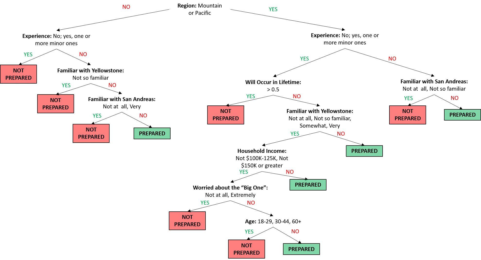
Now that we’ve built up our algorithm and split our data into training and test sets, let’s take a look at the full classification algorithm:
Recall the question we set out to answer with respect to the earthquake data: How well can we predict whether or not someone is prepared for an earthquake? In a binary (yes/no) case like this, we can set up our results in a 2x2 table, where the rows represent predicted preparedness (based on the features of our algorithm) and the columns represent true preparedness (what their true label is).

This simple 2x2 table carries quite a bit of information. Essentially, we can grade our machine on how well it learned to tell whether individuals are prepared or unprepared. We can see how well our algorithm did at classifying new observations by calculating the predictive accuracy, done by summing cells A and C and dividing by the total number of observations, or more simply, (A + C) / N. Through this calculation, we see that the algorithm from our example correctly classified individuals as prepared or unprepared 77.9% of the time. Not bad!
When we feed the roughly 500 test observations through the algorithm, it is the first time the machine has seen those observations. As a result, there is a chance that despite going through the algorithm, the machine misclassified someone as prepared, when in fact they were unprepared. To determine how often this happens, we can calculate the test error rate from the 2x2 table from above. To calculate the test error rate, we take the total number of observations that are discordant, or dissimilar between true and predicted status, and divide this total by the total number of observations that were assessed. Based on the above table, the test error rate would be (B + C) / N, or 22.1%.
There are a number of reasons that a test error rate would be high. Depending on the data set, there might be different methods that are better for developing the algorithm. Additionally, despite randomly splitting our data into training and testing sets, there may be some inherent differences between the two (think back to the employee income example above), making it harder for the algorithm to correctly label an observation.
References
Breiman, Leo, Jerome H Friedman, Richard A Olshen, and Charles J Stone. 1984. “Classification and Regression Trees. Wadsworth & Brooks.” Monterey, CA.
Hickey, Walt. 2015. “The Rock Isn’t Alone: Lots of People Are Worried About ‘the Big One’.” FiveThirtyEight. FiveThirtyEight. https://fivethirtyeight.com/datalab/the-rock-isnt-alone-lots-of-people-are-worried-about-the-big-one/.
Wikipedia. 2017a. “Earthquake — Wikipedia, the Free Encyclopedia.” http://en.wikipedia.org/w/index.php?title=Earthquake&oldid=762614740.
———. 2017b. “Predictive analytics — Wikipedia, the Free Encyclopedia.” http://en.wikipedia.org/w/index.php?title=Predictive%20analytics&oldid=764577274.
 Follow us on twitter